This is a re-post from my blog “SPM for programmers” which I am going to close in the next weeks. I thought, this is the most useful posting from there and worth keeping available.
What follows is a rough but hopefully didactically useful introduction into the neural model of DCM. The neural model does not aim to generate signals of single neurons or neuron populations but rather represents an abstract concept of how extrinsic input propagates through a network of brain areas. From this it follows, if no extrinsic signals enter the system, all brain areas remain in a stable state in terms of model parameters. Of course, the observed signals may contain all kinds of noise that are not modelled. For the sake of simplicity, in the following, we will discuss models which just consist of extrinsic signals entering the system and intrinsic connections between brain areas, but no bilinear influences. Thus, we reduce the well-known neuron model
to the form
where z is an n-dimensional vector representing the current neural states of n regions, u is a m-dimensional vector describing the extrinsic input of m sources entering the system, A is nxn-matrix describing the intrinsic connections between all regions, and C is a nxm-matrix depicting which region in the model is pertubed by extrinsic sources. The resulting vector ź indicates, in which direction the neural states have to be modified (also known as the first derivative of a function, modeling the neural states over time). The neural model of equation 1 is implemented in spm_fx_dcm.m, l. 64ff and l. 102ff.
In order to understand, how neural signals are computed and propagated through a network (without any theoretical knowledge about differential equations), let us assume a model with eight regions, in which region 1 is connected with region 2, region 2 with region 3, and so on until region 8 (fig. 1). The connection weights between all regions should be 1. Let us further assume, this model is driven by an external source that enters the network in region 1. This signal source is represented by a vector with T values. T is the number of time points for which we will generate the neural signal. (The value T depends on the number of scans, the TR and the temporal resolution for which the neural model should be generated. For example, the temporal resolution of the neural signal could be 1/16 = 0.0625 sec. For 200 scans at a TR of 2 secs, T would be 200×2×16 = 6400.) This external signal has the value 1 at the first time point followed by zeros. Put in simple words, we send a very short stimulus through the network and observe what happens.
The simulation starts with the neural states z = [0, 0, 0, 0, 0, 0, 0, 0], which means that no area has been influenced by a signal so far. For the first time point of the simulation of the neural signal, the equation given in 2 can be written as
One standard pre-assumption of the neural model of DCM is that each region has an inhibitory influence on itself. Therefore, the long diagonal of matrix A, which describes the influence each region exert on its own, contains -1. This is something, which is pre-specified and fix in any given DCM model. As the value -1 is multiplied with the signal intensity, the signal intensity in each region decays in each time step with a speed which is equal to its current intensity. In a few moments, we will see, what this actually means. Furthermore, each column of matrix A denotes for each region its connection strengths to other region. For example, the number in column one, row two gives us the information that region 1 propagates with strength 1 any signal to region 2. Accordingly, matrix C, which has eight rows (for eight regions) and one column (for one external input) specifies that signal u1 enters solely region 1. In the first time step u1 is, as defined, 1.
As the neural signal is modeled as continues signal, z1 is not simply z0 + ź1 but the activity that is continuously reached in the time that has passed between both time steps (e.g. 0.0625 secs). Therefore, the next state is exactly computed for any given time interval by solving the differential equation (spm_int.m, l. 164: x = spm_expm(J*dt(i),x);). The solution of equation 3 for a simulation period of 0.0625 secs returns the new state vector z1 ≈ [0.0606 0.0019, >0.0, >0.0, >0.0, >0.0, >0.0, >0.0]. All regions in z1 have already a value greater than zero as signal propagation is computed for all regions simultaneously.
In order to compute the next time point, we just have to replace z and u in equation 2 by the current values. Matrix A and C remain the same over the whole simulation time. Thus, the equation for the second time step is
Like in the previous step, the first derivatives for z2 are computed in the following way. For region 1: -1 * 0.0609 + 1 * 0 ≈ -0.0609. For region 2: 1*0.0609 + -1*0.0019 + 1*0 ≈ 0.0590. For region 3: 0 * 0.0609 + 1 * 0.0019 + -1 * >0.0 ≈ 0.0019. Again, as the neural signals are continues, the next time point after 0.0625 secs is also computed in a continuously manner by solving the differential equation. Thus, z2 ≈ [0.0569 0.0053 0.0003 >0.0 >0.0 >0.0 >0.0 >0.0].
Any further time steps are computed in the same way:
- Replace z and u in equation 2
- compute the derivative źt for time point t
- solve the differential equation for the current state
- compute the next neural state zt for a given time interval
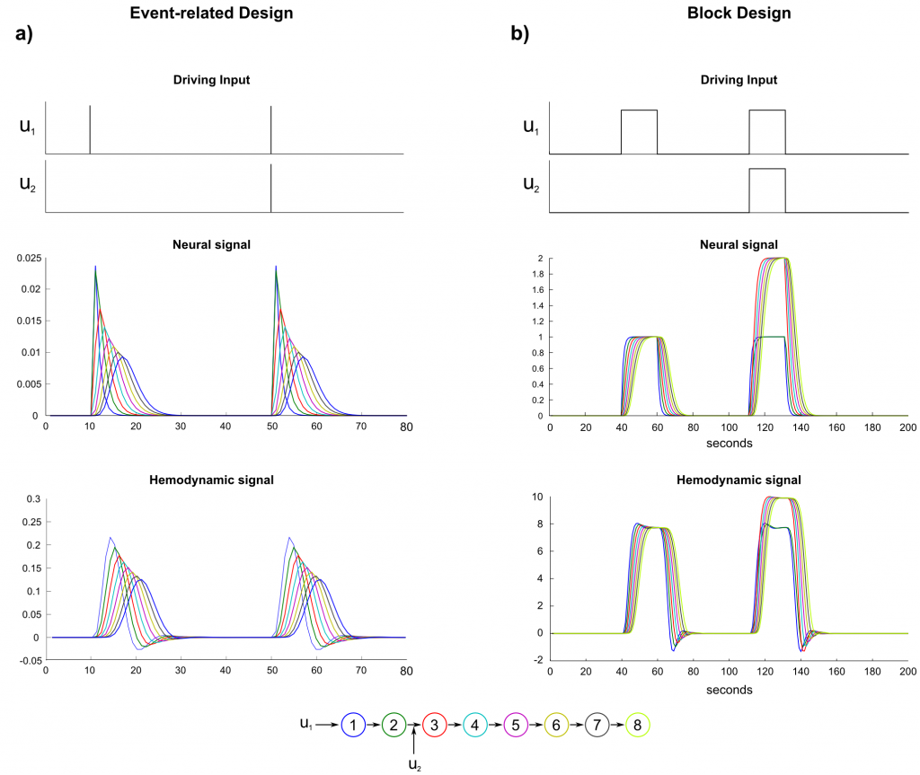
While the neural model is defined in spm_fx_dcm.m, the signal is generated in spm_int.m. The result of this simulation lasting for 20 secs is depicted in fig. 2. In other contexts, these signal courses are also called kernels, as they represent the basic function with which any external signal can be convolved in order to generate the neural signal. Figure 3 shows the neural signal for a block function as input.
Fig. 2: A stimulus function u (upper part of the image) enters a model with eight regions (lower part). The colored lines depict the neural signal that is generated for each region. The colors correspond to the regions displayed in the lower part of the image. x-axis: time in seconds, y-axis: activity in arbitrary scale.
Implications and interpretations
By estimating posterior probabilities for a given DCM, the researcher implicitly agrees, that neural signals which are propagated from region to region, can get delayed, smoother and weaker. This is an effect that is introduced by the neural model of DCM already and therefore can already be observed in the neural signal. As figure 3 shows, this holds also true for the neural signal affected by a block stimulus functions.
Fig. 3: A block stimulus u (upper part of the image) enters a model with eight regions (lower part). The colored lines depict the neural signal that is generated for each region. The colors correspond to the regions displayed in the lower part of the image. x-axis: time in seconds, y-axis: activity in arbitrary scale.
The observed delay and smoothing effect can be generated by two properties of the neural model of DCM: a scaling parameter determining the half-life of neural activity and the way neural activity is propagated through the network. The scaling parameter can be adjusted during the estimation process. A high value leads to a nearly loss-free propagation of a signal through all regions. However, when DCMs are generated using the spm_dcm_create-function (e.g. for testing the sensitivity of BMS) the parameter is set to zero, which we also used for our simulations and the depicted plots. The second factor that contributes to the observed delay in the neural signal is the neural model itself. A signal entering a dynamic system is not passed down from region to region like a package that is handed from person to person. Rather, regional activity just continuously increases by the activity of the preceding region comparable to a concatenation of pneumatic cylinders, while a self-inhibitory constant prevents the system from diverging to infinite values. Thus, a short stimulus causing a spike-like activation function in the first region generates expanding waves of activity in subsequent regions.
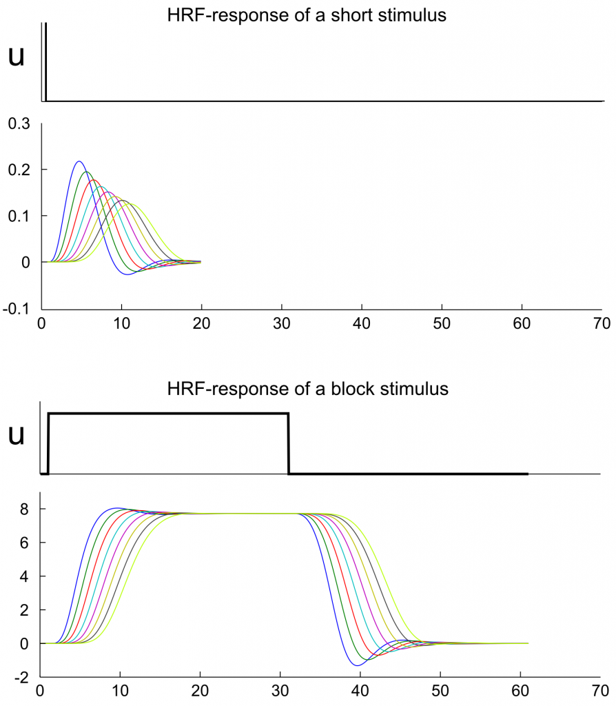
The implications of the neural model become apparent when the neural signal is converted into a hemodynamic response using the standard HRF-model of DCM (spm_gx_dcm.m) with the same standard HRF priors for each region (as given in spm_hdm_priors.m, l. 39, which are derived from the time courses of 128 voxels in the auditory cortex of a single subject (Friston et al. 1998, Friston et al. 2000)). Thus, we assured that any changes in form and delay can solely be attributed to the network definition and not to any changes of the HRF priors. Given, that all connection weights in the network are 1.0, the HRF responses reflect what should be observed when a signal enters the system and is propagated with a connection strength of 1.0 while at the same time each region inhibits itself with a strength of -1.0. Figure 4 depicts the hemodynamic response for a stick and block stimulus. The reader can generate the data with dcm_exp2.m (see below). The same effect can also be observed by generating a DCM with the spm_dcm_create-function which can be found in SPM5 and SPM8. (We recommend using a signal-to-noise ratio of 100 to see the effect without much noise. Alternatively, the user can set a breakpoint in spm_dcm_generate, right after the line y = feval (M.IS,P,M,U); to access the signal without any noise.)

Fig. 4: HRF-curves for the neuronal signals of figure 2 and 3. In this simulation it is assumed that all regions have the same hemodynamic priors. Any change in the form of the hemodynamic signal is therefore the implicit effect of the network configuration and the time scaling parameter. The plots can be reproduced with dcm_exp2.m (see below).
To interpret figure 4, the following explanations might help: The extrinsic input is propagated through the network without any lag (in terms of a time interval that passes before the signal starts to affect the next region). But the fact, that signal intensity in one region defines the increase of signal intensity in the next region, can generate a delay that sustains in the hemodynamic response. Therefore, each node in the model (fig. 4) reaches its peak activation with a delay of approximately one second compared to the previous node (This delay can also be seen in the upper right panel of figure 10 in Friston et al. 2003 but might be misleading as the x-axis is labeled with milliseconds instead of seconds.). We write “can generate”, because we used here the standard time scaling parameter of spm_dcm_create.m which is also the starting value in the estimation of a DCM. However, in the estimation procedure, this value can be adjusted to shorten this delay. With the term „delay“ we highlight post hoc a specific property of the kernel functions of the regions. One has to note, that each HRF-function has a specific form that depends on the network and hrf-parameters. In this regard, DCM does not directly introduce a delay in the signal but simulates signal propagation in a way that leads (among other differences) to a delayed signal peak in the HRF-response.
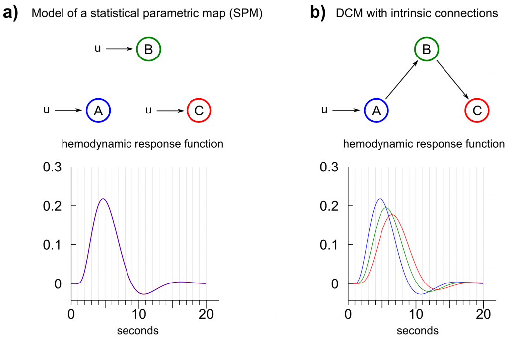
SPM represents a special case of DCM (Friston et al., 2003)â , since a DCM without any intrinsic connections, where input signals enter each region directly, would generate the regressors for a general linear model (This is not entirely true as the HRF-model of DCM differs slightly from the HRF-model used in SPM.). This means: By applying SPM, the user implicitly assumes that a signal entering the brain propagates fast enough through the whole network that simultaneity and a loss-free propagation can be assumed in order to find task-related regions (Of course, one can include the first derivative of the HRF-function to account for regional delays.). In contrast, in a DCM with signals propagating through intrinsic connections, model evidence is based upon a model fit which includes a propagated signal in regions that are driven by other regions (fig. 4). Thus, researchers have to be aware that using a SPM to select regions for a subsequent analysis with DCM means, that a certain a priori model and HRF-functions (e.g. fig. 5a) are used to select regions in order to apply another a priori model (e.g. fig. 5b) with potentially differing kernel-functions.

Fig. 5: Comparison between a dynamic causal model generating the regressors of a statistical parametric map (SPM) and a dynamic causal model where a signal enters a system in one region and propagates through the network by intrinsic connections. a) A SPM represents a special case of DCM where input enters each region directly and no intrinsic or bilinear connections are assumed. The hemodynamic response functions (HRFs) of all regions are identical given same HRF-priors for all regions. b) A typical setup for a dynamic causal model, in which a signal is propagated through intrinsic connections. The corresponding HRFs differ between regions given the same HRF-priors and the prior time scaling constant.
The effect of an external input modulating the connection between two regions with a strength of 1.0 is depicted in figure 6. In contrast to a direct influence on a region, a modulatory input increases the transition rate between two regions. In the given example, the connection between region 2 and 3 is increased from 1.0 to 2.0 during the contextual input of u2. When a block function is modulated by contextual input (fig. 6b), region 3 reaches its activation equilibrium between the driving input from region 2 and self-inhibition at 200% of the activation level of the former region. The hemodynamic model (again, we assume the same HRF-parameters for all regions) diminishes this effect down to ~120%.
In contrast, when a stick-functions of an event-related design is employed to modulate the connection between region 2 and 3, the modulatory effect is just applied for the fraction of a second invoking a very subtle difference between the unmodulated stimulus propagation and the modulated stimulus propagation. The difference becomes of course more pronounced, when the time scaling parameter is increased as the induced delay of the model gets lower. Nevertheless, a full modulatory influence between two regions during an event related stimulus presentation would only exist when the modulatory influence is modeled with a stimulus function that is active as long as there is activity in the driving region. This is the reason, why contextual input is usually modeled as block function.
 Fig. 6: Neural and hemodynamic signal of a model with bilinear connections. In an event-related design, the bilinear influence is comparatively lower than in a block design as the duration of the bilinear influence may not capture the duration in which a region drives another region. To account for a full bilinear influence, the bilinear regressor should be modeled as block-function (e.g. contextual condition).
Matlab code
Here are two demos (for SPM5 and early versions of SPM8) showing the neural- and hemodynamic signal in its noise-free form. The demos can be started with dcm_exp1 and dcm_exp2.
